#software for NPS distribution | Explore Tumblr posts and blogs

winsoftech · 2 years ago

Text

Revolutionising Wealth Management with Cutting-Edge Software Solutions

Introduction

In the ever-evolving banking and financial services landscape, staying ahead of the curve is imperative. One of the most groundbreaking advancements in this realm is integrating wealth management software. This innovative solution redefines how financial institutions operate and brings tangible benefits to both clients and professionals. In this article, we will delve into the transformative power of wealth management software, exploring its impact on banking and financial solutions and its role in NPS distribution.

The Power of Wealth Management Software

Enhancing Client Engagement

Gone are the days of endless paperwork and clunky spreadsheets. Wealth management software has ushered in a new era of streamlined interactions. Clients can now access their financial data, investment portfolios, and performance reports with just a few clicks. The user-friendly interface empowers clients to take control of their financial decisions, fostering a more profound sense of engagement and trust.

Optimising Financial Processes

Financial institutions are embracing the efficiency that comes with wealth management software. From automating routine tasks to real-time tracking of investment trends, these solutions bring a level of optimization that was once deemed unattainable. This reduces human error and frees up valuable time for financial professionals to focus on strategic, client-centric activities.

Banking and Financial Solutions in a New Light

Personalized Financial Planning

Wealth management software transcends one-size-fits-all approaches. It enables financial advisors to tailor their services to individual client needs. By analyzing intricate data points, such as spending habits and risk tolerance, the software assists in crafting personalized financial plans. This level of customization ensures that clients are on a trajectory to meet their unique financial goals.

Seamless Collaboration

In the collaborative world of finance, wealth management software shines. It allows financial advisors and clients to communicate seamlessly, regardless of geographical constraints. Through secure portals, clients can share important documents, ask questions, and receive expert real-time advice. This bridges the gap between professionals and clients, creating a holistic financial management experience.

Revolutionizing NPS Distribution

Navigating the Complexities

Software for NPS distribution brings unprecedented ease to an otherwise complex process. National Pension System (NPS) contributors can now track their investments, assess their fund performance, and receive updates effortlessly. This transparency empowers contributors and fosters a sense of security and confidence in the system.

Efficiency and Compliance

With regulatory landscapes becoming increasingly stringent, software solutions play a pivotal role in ensuring compliance. NPS distribution software automates compliance checks, reducing the risk of errors and penalties. Additionally, it accelerates the distribution process, ensuring that contributors receive their entitled benefits without unnecessary delays.

Conclusion

In the grand symphony of finance, the notes of innovation resonate loudly. Wealth management software harmonizes the complexities of banking and financial solutions with the intricacies of NPS distribution. As we embrace this technological revolution, companies like Winsoft Technologies and their pioneering software compose the melody of progress.

#NPS distribution software #wealth managment software #winsoft technologies

0 notes

redvision-technologies · 9 months ago

Text

How Does MF Back Office Software Help MFDs Handle Their Complex Business?

Handling the complex business of mutual fund distribution isn't easy, but many MFDs are turning to MF Back Office Software to make it a bit easier. The day-to-day operations of managing client portfolios, ensuring compliance, and maintaining a stable AUM can be overwhelming without the right tools.

Challenges for MFDs

Paper-Trail Onboarding: Traditional onboarding is slow and error-prone due to excessive paperwork, making it hard to manage and track client details.

Frequent Redemptions: Frequent client redemptions disrupt AUM, affecting revenue and requiring ongoing efforts to recover lost assets.

Declining AUM: A declining AUM impacts revenue and forces MFDs to focus on aggressive client acquisition, making long-term planning difficult.

Manual Workload: Relying on manual tasks like report generation and compliance checks increases workload and risks costly errors.

A Way to Overcome These Challenges

To overcome these challenges, MFDs are increasingly adopting mutual fund back office software in India, from REDVision Technologies, which offers a range of features designed to simplify and streamline operations. This software provides essential tools that help MFDs manage their business more efficiently and focus on growth.

Digital Onboarding

Digital onboarding replaces the traditional paper-based process with a streamlined, automated system that reduces errors and saves time. Clients can complete their onboarding process online, making it quicker and more convenient for both the MFD and the client.

Multiple Asset Management

It helps MFDs to offer multiple asset classes from a single platform. From Mutual Funds to IPOs, P2P, Equity, Global Investments, Loan Against Mutual Funds, and NPS, MFDs can offer everything through the same roof.

Automation

From automating report generation to scheduling reminders for due tasks, automation in software reduces the manual workload, minimizes errors, and ensures that all critical tasks are completed on time.

Automated Reporting and Due Alerts

With automated reporting, MFDs can generate accurate and timely reports with just a few clicks. They can also send due alerts on SIPs, FD maturity alerts, and more so that investors stay informed always.

Enhanced Client Communication

It also improves client communication by providing tools to send automated alerts, updates, and reports directly to clients. This ensures that clients are always informed about their investments, fostering trust and satisfaction.

Conclusion

There's nothing better than managing a complex business easily, and software helps them do it at their fingertips. If you haven't done it yet, it's time to give your business a spin.

#mutual fund software #mutual fund software for distributors #mutual fund software for ifa #mutual fund software in india #top mutual fund software in india #best mutual fund software in india #best mutual fund software #mutual fund software for distributors in india

0 notes

deploy111 · 1 year ago

Text

Task

This week’s assignment involves decision trees, and more specifically, classification trees. Decision trees are predictive models that allow for a data driven exploration of nonlinear relationships and interactions among many explanatory variables in predicting a response or target variable. When the response variable is categorical (two levels), the model is a called a classification tree. Explanatory variables can be either quantitative, categorical or both. Decision trees create segmentations or subgroups in the data, by applying a series of simple rules or criteria over and over again which choose variable constellations that best predict the response (i.e. target) variable.

Run a Classification Tree.

You will need to perform a decision tree analysis to test nonlinear relationships among a series of explanatory variables and a binary, categorical response variable.

Data

Features are computed from a digitized image of a fine needle aspirate (FNA) of a breast mass [K. P. Bennett and O. L. Mangasarian: "Robust Linear Programming Discrimination of Two Linearly Inseparable Sets", Optimization Methods and Software 1, 1992, 23-34].

Dataset can be found at UCI Machine Learning Repository

In this Assignment the Decision tree has been applied to classification of breast cancer detection.

Attribute Information:

id - ID number

diagnosis (M = malignant, B = benign)

3-32 extra features

Ten real-valued features are computed for each cell nucleus: a) radius (mean of distances from center to points on the perimeter) b) texture (standard deviation of gray-scale values) c) perimeter d) area e) smoothness (local variation in radius lengths) f) compactness (perimeter^2 / area - 1.0) g) concavity (severity of concave portions of the contour) h) concave points (number of concave portions of the contour) i) symmetry j) fractal dimension ("coastline approximation" - 1)

All feature values are recoded with four significant digits. Missing attribute values: none Class distribution: 357 benign, 212 malignant

Results

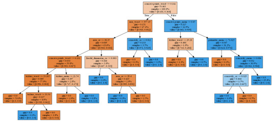
Generated decision tree can be found below:

In [17]:img

Out[17]:

Decision tree analysis was performed to test nonlinear relationships among a series of explanatory variables and a binary, categorical response variable (breast cancer diagnosis: malignant or benign).

The dataset was splitted into train and test samples in ratio 70\30.

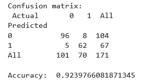
After fitting the classifier the key metrics were calculated - confusion matrix and accuracy = 0.924. This is a good result for a model trained on a small dataset.

From decision tree we can observe:

The malignant tumor is tend to have much more visible affected areas, texture and concave points, while the benign's characteristics are significantly lower.

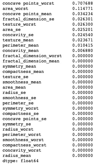
The most important features are:

concave points_worst = 0.707688

area_worst = 0.114771

concave points_mean = 0.034234

fractal_dimension_se = 0.026301

texture_worst = 0.026300

area_se = 0.025201

concavity_se = 0.024540

texture_mean = 0.023671

perimeter_mean = 0.010415

concavity_mean = 0.006880

Code

In [1]:import pandas as pd import numpy as np from sklearn.metrics import*from sklearn.model_selection import train_test_split from sklearn.tree import DecisionTreeClassifier from sklearn import tree from io import StringIO from IPython.display import Image import pydotplus from sklearn.manifold import TSNE from matplotlib import pyplot as plt %matplotlib inline rnd_state = 23468

Load data

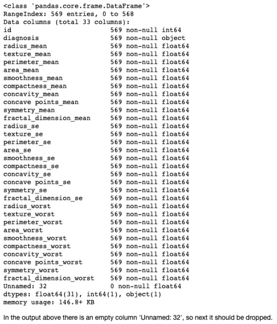
In [2]:data = pd.read_csv('Data/breast_cancer.csv') data.info() <class 'pandas.core.frame.DataFrame'> RangeIndex: 569 entries, 0 to 568 Data columns (total 33 columns): id 569 non-null int64 diagnosis 569 non-null object radius_mean 569 non-null float64 texture_mean 569 non-null float64 perimeter_mean 569 non-null float64 area_mean 569 non-null float64 smoothness_mean 569 non-null float64 compactness_mean 569 non-null float64 concavity_mean 569 non-null float64 concave points_mean 569 non-null float64 symmetry_mean 569 non-null float64 fractal_dimension_mean 569 non-null float64 radius_se 569 non-null float64 texture_se 569 non-null float64 perimeter_se 569 non-null float64 area_se 569 non-null float64 smoothness_se 569 non-null float64 compactness_se 569 non-null float64 concavity_se 569 non-null float64 concave points_se 569 non-null float64 symmetry_se 569 non-null float64 fractal_dimension_se 569 non-null float64 radius_worst 569 non-null float64 texture_worst 569 non-null float64 perimeter_worst 569 non-null float64 area_worst 569 non-null float64 smoothness_worst 569 non-null float64 compactness_worst 569 non-null float64 concavity_worst 569 non-null float64 concave points_worst 569 non-null float64 symmetry_worst 569 non-null float64 fractal_dimension_worst 569 non-null float64 Unnamed: 32 0 non-null float64 dtypes: float64(31), int64(1), object(1) memory usage: 146.8+ KB

In the output above there is an empty column 'Unnamed: 32', so next it should be dropped.

In [3]:data.drop('Unnamed: 32', axis=1, inplace=True) data.diagnosis = np.where(data.diagnosis=='M', 1, 0) # Decode diagnosis into binary data.describe()

Out[3]:iddiagnosisradius_meantexture_meanperimeter_meanarea_meansmoothness_meancompactness_meanconcavity_meanconcave points_mean...radius_worsttexture_worstperimeter_worstarea_worstsmoothness_worstcompactness_worstconcavity_worstconcave points_worstsymmetry_worstfractal_dimension_worstcount5.690000e+02569.000000569.000000569.000000569.000000569.000000569.000000569.000000569.000000569.000000...569.000000569.000000569.000000569.000000569.000000569.000000569.000000569.000000569.000000569.000000mean3.037183e+070.37258314.12729219.28964991.969033654.8891040.0963600.1043410.0887990.048919...16.26919025.677223107.261213880.5831280.1323690.2542650.2721880.1146060.2900760.083946std1.250206e+080.4839183.5240494.30103624.298981351.9141290.0140640.0528130.0797200.038803...4.8332426.14625833.602542569.3569930.0228320.1573360.2086240.0657320.0618670.018061min8.670000e+030.0000006.9810009.71000043.790000143.5000000.0526300.0193800.0000000.000000...7.93000012.02000050.410000185.2000000.0711700.0272900.0000000.0000000.1565000.05504025%8.692180e+050.00000011.70000016.17000075.170000420.3000000.0863700.0649200.0295600.020310...13.01000021.08000084.110000515.3000000.1166000.1472000.1145000.0649300.2504000.07146050%9.060240e+050.00000013.37000018.84000086.240000551.1000000.0958700.0926300.0615400.033500...14.97000025.41000097.660000686.5000000.1313000.2119000.2267000.0999300.2822000.08004075%8.813129e+061.00000015.78000021.800000104.100000782.7000000.1053000.1304000.1307000.074000...18.79000029.720000125.4000001084.0000000.1460000.3391000.3829000.1614000.3179000.092080max9.113205e+081.00000028.11000039.280000188.5000002501.0000000.1634000.3454000.4268000.201200...36.04000049.540000251.2000004254.0000000.2226001.0580001.2520000.2910000.6638000.207500

8 rows × 32 columns

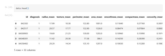
In [4]:data.head()

Out[4]:iddiagnosisradius_meantexture_meanperimeter_meanarea_meansmoothness_meancompactness_meanconcavity_meanconcave points_mean...radius_worsttexture_worstperimeter_worstarea_worstsmoothness_worstcompactness_worstconcavity_worstconcave points_worstsymmetry_worstfractal_dimension_worst0842302117.9910.38122.801001.00.118400.277600.30010.14710...25.3817.33184.602019.00.16220.66560.71190.26540.46010.118901842517120.5717.77132.901326.00.084740.078640.08690.07017...24.9923.41158.801956.00.12380.18660.24160.18600.27500.08902284300903119.6921.25130.001203.00.109600.159900.19740.12790...23.5725.53152.501709.00.14440.42450.45040.24300.36130.08758384348301111.4220.3877.58386.10.142500.283900.24140.10520...14.9126.5098.87567.70.20980.86630.68690.25750.66380.17300484358402120.2914.34135.101297.00.100300.132800.19800.10430...22.5416.67152.201575.00.13740.20500.40000.16250.23640.07678

5 rows × 32 columns

Plots

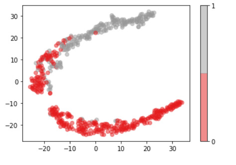
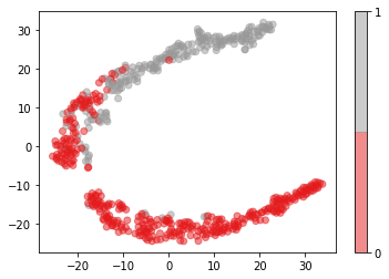
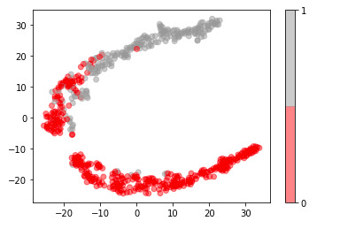
For visualization purposes, the number of dimensions was reduced to two by applying t-SNE method. The plot illustrates that our classes are not clearly divided into two parts, so the nonlinear methods (like Decision tree) may solve this problem.

In [15]:model = TSNE(random_state=rnd_state, n_components=2) representation = model.fit_transform(data.iloc[:, 2:])

In [16]:plt.scatter(representation[:, 0], representation[:, 1], c=data.diagnosis, alpha=0.5, cmap=plt.cm.get_cmap('Set1', 2)) plt.colorbar(ticks=range(2));

Decision tree

In [6]:predictors = data.iloc[:, 2:] target = data.diagnosis

To train a Decision tree the dataset was splitted into train and test samples in proportion 70/30.

In [7]:(predictors_train, predictors_test, target_train, target_test) = train_test_split(predictors, target, test_size = .3, random_state = rnd_state)

In [8]:print('predictors_train:', predictors_train.shape) print('predictors_test:', predictors_test.shape) print('target_train:', target_train.shape) print('target_test:', target_test.shape) predictors_train: (398, 30) predictors_test: (171, 30) target_train: (398,) target_test: (171,)

In [9]:print(np.sum(target_train==0)) print(np.sum(target_train==1)) 253 145

Our train sample is quite balanced, so there is no need in balancing it.

In [10]:classifier = DecisionTreeClassifier(random_state = rnd_state).fit(predictors_train, target_train)

In [11]:prediction = classifier.predict(predictors_test)

In [12]:print('Confusion matrix:\n', pd.crosstab(target_test, prediction, colnames=['Actual'], rownames=['Predicted'], margins=True)) print('\nAccuracy: ', accuracy_score(target_test, prediction)) Confusion matrix: Actual 0 1 All Predicted 0 96 8 104 1 5 62 67 All 101 70 171 Accuracy: 0.9239766081871345

In [13]:out = StringIO() tree.export_graphviz(classifier, out_file = out, feature_names = predictors_train.columns.values, proportion =True, filled =True) graph = pydotplus.graph_from_dot_data(out.getvalue()) img = Image(data = graph.create_png()) with open('output.png', 'wb') as f: f.write(img.data)

In [14]:feature_importance = pd.Series(classifier.feature_importances_, index=data.columns.values[2:]).sort_values(ascending=False) feature_importance

Out[14]:concave points_worst 0.707688 area_worst 0.114771 concave points_mean 0.034234 fractal_dimension_se 0.026301 texture_worst 0.026300 area_se 0.025201 concavity_se 0.024540 texture_mean 0.023671 perimeter_mean 0.010415 concavity_mean 0.006880 fractal_dimension_worst 0.000000 fractal_dimension_mean 0.000000 symmetry_mean 0.000000 compactness_mean 0.000000 texture_se 0.000000 smoothness_mean 0.000000 area_mean 0.000000 radius_se 0.000000 smoothness_se 0.000000 perimeter_se 0.000000 symmetry_worst 0.000000 compactness_se 0.000000 concave points_se 0.000000 symmetry_se 0.000000 radius_worst 0.000000 perimeter_worst 0.000000 smoothness_worst 0.000000 compactness_worst 0.000000 concavity_worst 0.000000 radius_mean 0.000000 dtype: float64

0 notes

survey2connectsposts · 2 years ago

Text

Best NPS Survey Tools & Software for 2023 | Survey2Connect

Survey2Connect is a great NPS Survey tool that can create NPS Surveys and send them to your customers through multiple channels to measure customer loyalty and satisfaction. It notifies you of detractors, collects actionable feedback, works on it, closes the feedback loop, and converts your detractors into promoters. It’s easy to use and offers customizable survey templates, making it easier to create and distribute NPS surveys.

#NPS_Survey_tools #Net_Promoter_Score_Tool

0 notes

data-analysis21 · 2 years ago

Text

Running a Classification Tree

This week’s assignment involves decision trees, and more specifically, classification trees. Decision trees are predictive models that allow for a data driven exploration of nonlinear relationships and interactions among many explanatory variables in predicting a response or target variable. When the response variable is categorical (two levels), the model is a called a classification tree. Explanatory variables can be either quantitative, categorical or both. Decision trees create segmentation or subgroups in the data, by applying a series of simple rules or criteria over and over again which choose variable constellations that best predict the response (i.e. target) variable.

Run a Classification Tree.

Data

In this Assignment the Decision tree has been applied to classification of breast cancer detection.

Attribute Information:

id - ID number

diagnosis (M = malignant, B = benign)

3-32 extra features

All feature values are recorded with four significant digits. Missing attribute values: none Class distribution: 357 benign, 212 malignant

Results

Generated decision tree can be found below:

The dataset was splitted into train and test samples in ratio 70\30.

After fitting the classifier the key metrics were calculated - confusion matrix and accuracy = 0.924. This is a good result for a model trained on a small dataset.

From decision tree we can observe:

The malignant tumor is tend to have much more visible affected areas, texture and concave points, while the benign's characteristics are significantly lower.

The most important features are:

concave points_worst = 0.707688

area_worst = 0.114771

concave points_mean = 0.034234

fractal_dimension_se = 0.026301

texture_worst = 0.026300

area_se = 0.025201

concavity_se = 0.024540

texture_mean = 0.023671

perimeter_mean = 0.010415

concavity_mean = 0.006880

Code

import pandas as pd

import numpy as np

from sklearn.metrics import * from sklearn.model_selection

import train_test_split from sklearn.tree

import DecisionTreeClassifier

from sklearn import tree

from io import StringIO

from IPython.display import Image

import pydotplus

from sklearn.manifold import TSNE

from matplotlib import pyplot as plt

%matplotlib inline

rnd_state = 23467

Load data

data = pd.read_csv('Data/breast_cancer.csv')

data.info()

Output:

<class 'pandas.core.frame.DataFrame'> RangeIndex: 569 entries, 0 to 568 Data columns (total 33 columns): id 569 non-null int64 diagnosis 569 non-null object radius_mean 569 non-null float64 texture_mean 569 non-null float64 perimeter_mean 569 non-null float64 area_mean 569 non-null float64 smoothness_mean 569 non-null float64 compactness_mean 569 non-null float64 concavity_mean 569 non-null float64 concave points_mean 569 non-null float64 symmetry_mean 569 non-null float64 fractal_dimension_mean 569 non-null float64 radius_se 569 non-null float64 texture_se 569 non-null float64 perimeter_se 569 non-null float64 area_se 569 non-null float64 smoothness_se 569 non-null float64 compactness_se 569 non-null float64 concavity_se 569 non-null float64 concave points_se 569 non-null float64 symmetry_se 569 non-null float64 fractal_dimension_se 569 non-null float64 radius_worst 569 non-null float64 texture_worst 569 non-null float64 perimeter_worst 569 non-null float64 area_worst 569 non-null float64 smoothness_worst 569 non-null float64 compactness_worst 569 non-null float64 concavity_worst 569 non-null float64 concave points_worst 569 non-null float64 symmetry_worst 569 non-null float64 fractal_dimension_worst 569 non-null float64 Unnamed: 32 0 non-null float64 dtypes: float64(31), int64(1), object(1) memory usage: 146.8+ KB

In the output above there is an empty column 'Unnamed: 32', so next it should be dropped.

Plots

model = TSNE(random_state=rnd_state, n_components=2) representation = model.fit_transform(data.iloc[:, 2:])

plt.scatter(representation[:, 0], representation[:, 1], c=data.diagnosis, alpha=0.5, cmap=plt.cm.get_cmap('Set1', 2)) plt.colorbar(ticks=range(2));

Decision tree

predictors = data.iloc[:, 2:]

target = data.diagnosis

To train a Decision tree the dataset was splitted into train and test samples in proportion 70/30.

(predictors_train, predictors_test, target_train, target_test) = train_test_split(predictors, target, test_size = .3, random_state = rnd_state)

print('predictors_train:', predictors_train.shape) print('predictors_test:', predictors_test.shape) print('target_train:', target_train.shape) print('target_test:', target_test.shape)

Output:

predictors_train: (398, 30)

predictors_test: (171, 30)

target_train: (398,)

target_test: (171,)

print(np.sum(target_train==0))

print(np.sum(target_train==1))

Output:

253

145

Our train sample is quite balanced, so there is no need in balancing it.

classifier = DecisionTreeClassifier(random_state = rnd_state).fit(predictors_train, target_train)

prediction = classifier.predict(predictors_test)

print('Confusion matrix:\n', pd.crosstab(target_test, prediction, colnames=['Actual'], rownames=['Predicted'], margins=True)) print('\nAccuracy: ', accuracy_score(target_test, prediction))

out = StringIO() tree.export_graphviz(classifier, out_file = out, feature_names = predictors_train.columns.values, proportion = True, filled = True) graph = pydotplus.graph_from_dot_data(out.getvalue()) img = Image(data = graph.create_png()) with open('output.png', 'wb') as f: f.write(img.data)

feature_importance = pd.Series(classifier.feature_importances_, index=data.columns.values[2:]).sort_values(ascending=False) feature_importance

concave points_worst 0.705688 area_worst 0.214871 concave points_mean 0.034234 fractal_dimension_se 0.028301 texture_worst 0.026300 area_se 0.025201 concavity_se 0.024540 texture_mean 0.023671 perimeter_mean 0.010415 concavity_mean 0.006880 fractal_dimension_worst 0.000000 fractal_dimension_mean 0.000000 symmetry_mean 0.000002 compactness_mean 0.005000 texture_se 0.000000 smoothness_mean 0.000000 area_mean 0.000000 radius_se 0.000000 smoothness_se 0.000000 perimeter_se 0.000001 symmetry_worst 0.000000 compactness_se 0.000000 concave points_se 0.000000 symmetry_se 0.000000 radius_worst 0.000000 perimeter_worst 0.000000 smoothness_worst 0.000000 compactness_worst 0.000002 concavity_worst 0.000000 radius_mean 0.000000 dtype: float64

#decision tree

1 note · View note

healthkenya7 · 2 years ago

Text

ADVANCEMENTS IN BRAIN IMAGING FOR EARLY DEMENTIA DETECTION

Advancements in brain imaging techniques have significantly contributed to the early detection and understanding of dementia. Dementia is a progressive neurodegenerative disorder characterized by cognitive decline, memory loss, impaired reasoning, and other cognitive deficits. Detecting dementia at an early stage is crucial for effective intervention and management. Various imaging modalities have been developed and refined to provide detailed insights into brain structure, function, and connectivity, aiding in the early detection of dementia. Below, we explore some of the key advancements in brain imaging for early dementia detection:

Structural MRI (magnetic resonance imaging): Structural MRI provides detailed images of brain anatomy and can detect changes in brain volume and tissue composition. Advanced techniques such as voxel-based morphometry (VBM) allow for the analysis of regional brain volume changes over time. In dementia, regions like the hippocampus and cortex often show atrophy in early stages. Automated software tools help identify subtle changes and compare an individual's brain structure to a normative database.

Functional MRI (fMRI): fMRI measures changes in blood flow and oxygenation to infer brain activity. Resting-state fMRI can reveal functional connectivity patterns between different brain regions. Alterations in functional connectivity networks are linked to early dementia stages. Researchers use various analysis methods like independent component analysis (ICA) and seed-based correlation to identify disrupted connectivity related to memory, attention, and executive function.

Diffusion MRI: Diffusion MRI captures the movement of water molecules in brain tissue, providing information about white matter integrity and connectivity. Diffusion tensor imaging (DTI) and more advanced techniques like diffusion kurtosis imaging (DKI) allow the mapping of white matter microstructure changes, which can indicate early signs of neurodegeneration in dementia.

PET (positron emission tomography): PET scans can track specific molecules in the brain, such as glucose metabolism and amyloid-beta plaques, which are associated with Alzheimer's disease. F-18 FDG PET measures glucose uptake, reflecting neuronal activity and metabolism. Amyloid PET tracers, like florbetapir and flutemetamol, bind to amyloid plaques, helping diagnose Alzheimer's disease.

SPECT (single-photon emission computed tomography): SPECT is another nuclear imaging technique used to measure blood flow in the brain. It can help identify regional cerebral blood flow abnormalities and is particularly useful in distinguishing between different types of dementia, such as Alzheimer's disease and frontotemporal dementia.

Molecular Imaging: Emerging techniques like tau PET imaging are designed to detect tau protein aggregates, which are another hallmark of Alzheimer's disease. Tau PET scans provide insight into the distribution and severity of tau pathology in the brain.

Machine Learning and AI: Advanced data analysis methods, particularly machine learning and artificial intelligence (AI), have transformed brain imaging for dementia detection. These techniques can identify subtle patterns and predict disease progression based on imaging data. AI algorithms trained on large datasets can enhance diagnostic accuracy and aid in personalized treatment strategies.

Mr. Jayesh Saini says, “Advancements in brain imaging have revolutionized our ability to detect and understand early-stage dementia. These imaging modalities provide valuable insights into structural, functional, and molecular changes in the brain, helping clinicians diagnose dementia at an earlier stage and enabling researchers to develop better treatments and interventions for affected individuals.”

#jayeshsaini #healthcare #LifeCareHospitals #Kenya #NHIF #NPS #TSC#healthy

0 notes

salwari · 2 years ago

Text

How-often-should-I-survey-the-net-promoter-score-NPS

Net Promoter Score (NPS) has become a key metric for businesses to measure customer loyalty and satisfaction. NPS surveys gauge how likely customers are to recommend a company’s products or services to others, providing valuable insights into the overall customer experience. However, the frequency of conducting NPS surveys is a critical consideration. It’s essential to strike a balance between gathering sufficient data and avoiding survey fatigue. In this article, we’ll explore the factors to consider when determining how often to conduct NPS surveys, the role of NPS survey software, other NPS survey tools, and NPS survey platforms in achieving survey success.

Survey Goals and Customer Lifecycle: The frequency of NPS surveys should align with the goals of the survey and the stage of the customer lifecycle. For instance, if the primary objective is to track long-term customer satisfaction, conducting quarterly or bi-annual NPS surveys may be appropriate. On the other hand, if the focus is on evaluating the customer experience after a specific interaction, such as a purchase or support request, more frequent surveys, such as after each transaction, might be necessary.

Sampling Methodology: The size and composition of your customer base also play a role in determining survey frequency. For businesses with a large and diverse customer pool, conducting periodic surveys might suffice. However, for smaller businesses with a more focused customer base, more frequent surveys may be needed to capture meaningful feedback from a representative sample.

Seasonal or Event-Driven Considerations: Certain businesses experience fluctuations in customer activity due to seasonal trends or events. For example, a travel company might observe higher customer engagement during the holiday season. In such cases, adjusting the survey frequency to coincide with peak or low periods can provide valuable insights into customer sentiment during specific times.

Response and Actionability: It’s essential to give your organization enough time to process and act upon the feedback gathered from NPS surveys. If you overwhelm your team with a high frequency of surveys, they may struggle to take meaningful action based on the results. Strike a balance to ensure that the software or platforms you use provide sufficient time for analysis and implementation of improvements between survey cycles.

Competitive Analysis: Comparing your NPS scores with those of your competitors can offer valuable benchmarks and insights into your relative performance. If your competitors conduct NPS surveys at specific intervals, it may be beneficial to align your survey frequency accordingly for more accurate comparisons.

Utilizing the best NPS software, or other survey tools and platforms can significantly streamline the survey process. These tools often offer automated survey distribution, real-time data analysis, and customizable reporting, making it easier to gather, analyze, and act upon customer feedback effectively.

In conclusion, determining the ideal frequency for the best NPS survey tools requires a thoughtful approach. Align your survey frequency with your goals, customer lifecycle, and sampling needs while considering seasonal variations. Strive for a balance that provides actionable insights without overwhelming your team or customers.

#Nps Survey #Nps Survey Tool #Nps Survey Software #Survey Tool

0 notes

techgizmohub · 2 years ago

Link

#3DPrint.com #Capabilities #Gizmo #Hub #InFlight #Marines #MV22 #Ospreys #Printing #Report #Showcase #tech

0 notes

craigbrownphd · 3 years ago

Text

If you did not already know

Ensemble Feature Selection Integrating Stability (EFSIS) Ensemble learning that can be used to combine the predictions from multiple learners has been widely applied in pattern recognition, and has been reported to be more robust and accurate than the individual learners. This ensemble logic has recently also been more applied in feature selection. There are basically two strategies for ensemble feature selection, namely data perturbation and function perturbation. Data perturbation performs feature selection on data subsets sampled from the original dataset and then selects the features consistently ranked highly across those data subsets. This has been found to improve both the stability of the selector and the prediction accuracy for a classifier. Function perturbation frees the user from having to decide on the most appropriate selector for any given situation and works by aggregating multiple selectors. This has been found to maintain or improve classification performance. Here we propose a framework, EFSIS, combining these two strategies. Empirical results indicate that EFSIS gives both high prediction accuracy and stability. … Learning to Weight (LTW) In information retrieval (IR) and related tasks, term weighting approaches typically consider the frequency of the term in the document and in the collection in order to compute a score reflecting the importance of the term for the document. In tasks characterized by the presence of training data (such as text classification) it seems logical that the term weighting function should take into account the distribution (as estimated from training data) of the term across the classes of interest. Although `supervised term weighting’ approaches that use this intuition have been described before, they have failed to show consistent improvements. In this article we analyse the possible reasons for this failure, and call consolidated assumptions into question. Following this criticism we propose a novel supervised term weighting approach that, instead of relying on any predefined formula, learns a term weighting function optimised on the training set of interest; we dub this approach \emph{Learning to Weight} (LTW). The experiments that we run on several well-known benchmarks, and using different learning methods, show that our method outperforms previous term weighting approaches in text classification. … International Institute for Analytics (IIA) Founded in 2010 by CEO Jack Phillips and Research Director Thomas H. Davenport, the International Institute for Analytics is an independent research firm that works with organizations to build strong and competitive analytics programs. IIA offers unbiased advice in an industry dominated by hardware and software vendors, consultants and system integrators. With a vast network of analytics experts, academics and leaders at successful companies, we guide our clients as they build and grow successful analytics programs. … Answer Set Programming (ASP) Answer set programming (ASP) is a form of declarative programming oriented towards difficult (primarily NP-hard) search problems. It is based on the stable model (answer set) semantics of logic programming. In ASP, search problems are reduced to computing stable models, and answer set solvers – programs for generating stable models – are used to perform search. The computational process employed in the design of many answer set solvers is an enhancement of the DPLL algorithm and, in principle, it always terminates (unlike Prolog query evaluation, which may lead to an infinite loop). In a more general sense, ASP includes all applications of answer sets to knowledge representation and the use of Prolog-style query evaluation for solving problems arising in these applications. The Seventh Answer Set Programming Competition: Design and Results … https://analytixon.com/2022/07/30/if-you-did-not-already-know-1789/?utm_source=dlvr.it&utm_medium=tumblr

2 notes · View notes

recruitingjobsincanada · 4 years ago

Text

Recruiting Jobs In Canada

Are you seeking out Recruiting Jobs In Canada for the employment carrier in 2021? Or, do you want a job consultancy carrier in Canada? If sure, then accurate information for you. To get a higher task and employment provider to your favourite vicinity like Toronto, Vancouver, Edmonton, Calgary and lots of extra. They are the pinnacle and high-quality recruiters in Canada in 2021.

if you are attempting to find jobs in Canada for foreigners, then those recruitment employers in Canada will assist you to discover the nice jobs for you in the favored vicinity.

The primary factor extra complex than getting the right staffing and skills in Canada is dealing with employment arrangements for foreign people. Canada has visible sizable increase in the infrastructure, power, improvement and method industries in recent years.

That increase has generated massive demand for exceedingly knowledgeable, trained and skilled specialists, which include engineers, executives, researchers, chemists, and architects.

There has been an growth in Canadian employers hiring foreign people for those skilled and regularly revel in-intensive positions. it may be hard to locate the right recruiters and expertise.

Why to seek advice from an Employment organisation to discover a job?

In keeping with the survey, extra than ninety percentage of agencies in Canada use recruitment businesses to lease personnel. Recruiting consultancy to play a mediator role in assisting organizations to discover the satisfactory skills and people to discover the right job.

In contrast to company recruiters, recruiters at hiring corporations have access to all forms of jobs at multiple businesses protecting an extensive spectrum of industries and task positions. If corporations and your opposition are the use of them, you must be too. Right here are a few points of motives to seek advice from an employment employer for both the employers and task seekers.

CAN save you TIME AND stress

try OUT JOBS earlier than YOU commit

potential FOR more options

IT’S less complicated to say NO

only practice TO serious businesses trying to lease

REPRESENTATIVES ARE notably inspired TO GET YOU positioned

THEY recognize THE proper human beings

help AND assist

At secondary 10 careers of the destiny school and college graduations, it’s entirely expected to listen to an audio system asking children to follow their passion. The notion is that inside the occasion that you attempt to earn sufficient to pay the payments carrying out something you adore, you’ll paintings greater diligently at it, and achievement and flourishing will follow.

but in truth, it doesn’t typically workout that manner. At the off chance that the field you feel generally active about is in decay, like journalism, seeking after it is able to imply severa long durations of battle, definitely attempting to get and maintain a line of labor. also, if the positions you’re ready to find out don’t pay a living pay, you could revel in taking care of the bills on any occasion, when you’re applied.

software program Developer

software program engineers plan and compose the product that sudden spikes in call for devices like computers and smartphones. a few engineers make programs for precise duties, while others paintings on the working frameworks used by networks and working structures. Software improvement consists of finding out what customers need, making plans and trying out software to deal with the ones troubles, making actions up to greater hooked up tasks, and maintaining up and documenting the software improvement technique to make certain it maintains to work efficiently afterward.

scientific and fitness offerings manager

hospital therapy is a main and convoluted business. Giving attention to patients is simply critical for it. There’s additionally paintings of making plans preparations, gathering payments, retaining clinical records, and organizing with different fitness offerings companies. clinical and fitness managers regulate each such sporting event, leaving medical care companies with greater possibilities for their sufferers.

Postsecondary instructor

Any trainer who teaches students beyond the excessive college level may be termed as a postsecondary teacher. 10 careers of destiny those teachers can teach any problem but the demand is rising speedy for scientific, commercial enterprise, and nursing teachers. alongside teaching lessons, postsecondary teachers often take part in studies, distribute books and papers, and set off students about choosing a university foremost and accomplishing their expert goals.

Nurse Practitioner

A nurse practitioner, or NP, is a type of nurse with greater instruction and more authority than a registered nurse (RN). in place of honestly helping experts, NPs can carry out a full-size lot of a consultant’s capacities themselves. A NP can analyze illnesses, advise meds, and deal with an affected person’s trendy attention.

financial supervisor

Each employer, from a nook supermarket to a Fortune 500 company, wishes to manage cash. at the off chance that the commercial enterprise is adequately huge, it would hire a financial manager to manipulate that facet of the commercial enterprise. The financial supervisor monitors an affiliation’s pay and spending, looking for processes to amplify advantages and diminish expenses. They make monetary reviews, oversee ventures, and help direct the affiliation’s drawn-out economic targets.

management Analyst

management professionals, in any other case referred to as management specialists, help companies discover approaches to run all of the more proficiently. they arrive into an enterprise and note its methods, speak with a team of workers, and have a look at economic statistics. At that point, they encourage supervisors at the maximum talented technique to lower charges (for example, by using the same paintings with much less fee) or lift earning (as an example, by using expanding the degree of an object an organisation can supply in a day).

physical Therapist

physical therapists help people with wounds or sicknesses that cause ache and affect motion. They use techniques like stretches or distinctive sports and body control to assist patients with enhancing their portability and lessen torment.

creation manager

On the point when you pass a creation site, you often see severa production workers fascinated by the involved profession of a building. creation supervisors aren’t commonly obvious on the scene, but, they’re generally there in the back of it. From taking into consideration the underlying rate issue to directing people to make certain the work is up to code, they’re associated with each segment of the shape cycle.

statistics security Analyst

groups rent statistics safety analysts to guard their laptop networks and frameworks from cybercrime. Those professionals introduce antivirus programming and distinct shields to make certain records are being covered, look ahead to protection penetrates and examine them once they show up and intermittently take a look at the community to look for holes a programmer should abuse. They likewise make recovery plans that intend to assist the networks with getting their framework operating within the event of an assault. Which could consist of removing harmful software programs from the computers and reestablishing statistics from backups.

laptop and information structures supervisor

A pc and records frameworks manager is answerable for all the laptop-associated sporting events inner an organization or other association. The paintings can include analyzing pc desires, prescribing actions as much as the framework, introducing and keeping up computers and programming, and coordinating other laptop-related experts, like programming engineers and records protection investigators.

#Recruiting Jobs In Canada

1 note · View note

winsoftech · 2 years ago

Text

Transforming Banking and Financial Solutions with Innovative Software for NPS Distribution

Banking and financial institutions constantly seek new ways to upscale their services and enhance customer experience. One area that has witnessed significant transformation in recent years is the distribution of National Pension System (NPS) products. With the advent of cutting-edge software for NPS distribution, such as those offered by Winsoft Technologies, the industry has been revolutionised, offering unprecedented convenience, efficiency and security.

The Evolution of NPS Distribution

Traditionally, NPS distribution involved manual processes, cumbersome paperwork, and lengthy turnaround times. This created challenges for both customers and financial institutions and limited the reach and accessibility of these valuable products. However, the landscape has dramatically changed with the introduction of advanced software solutions.

Streamlined Operations and Enhanced Efficiency

One of the key benefits of leveraging software for NPS distribution is the streamlining of operations. With intuitive interfaces, automated workflows, and seamless integration with existing systems, banks and financial institutions can significantly enhance their operational efficiency. This enables them to process applications faster, reduce errors, and improve overall customer satisfaction.

Superior Customer Experience

In today's digital age, customers demand convenience and personalised experiences and software for NPS distribution enables financial institutions to provide just that. With user-friendly interfaces and self-service options, customers can easily explore NPS products, access real-time information, and initiate transactions at their convenience. This empowers them enabling them to make informed decisions and control their financial future.

Robust Security Measures

Security is a paramount concern in the banking and financial sector, and rightly so. Software solutions for NPS distribution prioritise data protection and implement stringent security measures. Through encryption, secure authentication protocols, and regular audits, these solutions safeguard sensitive customer information from unauthorised access and potential threats. This instils confidence in customers and enhances trust in the institution.

Enhancing Accessibility through Mobile Applications

In today's mobile-driven world, accessibility is vital to staying competitive in the banking and financial sector. Software solutions for NPS distribution offered by Winsoft Technologies have considered this by incorporating mobile applications into their offerings. These applications enable customers to access their NPS accounts anytime, anywhere, using their smartphones or tablets.

With features like balance inquiries, fund transfers, and transaction history, customers have complete control over their NPS investments on the go. This level of accessibility ensures that customers can manage their financial future effortlessly, further solidifying Winsoft Technologies' position as an industry leader.

#software for NPS distribution #Winsoft Technologies

0 notes

priteshchhabra · 5 years ago

Text

Peer-graded Assignment: Running a Classification Tree

Data

Dataset can be found at UCI Machine Learning Repository

In this Assignment the Decision tree has been applied to classification of breast cancer detection.

Attribute Information:

id - ID number

diagnosis (M = malignant, B = benign)

3-32 extra features

All feature values are recoded with four significant digits. Missing attribute values: none Class distribution: 357 benign, 212 malignant

Results

Generated decision tree can be found below:

In [17]:

img

Out[17]:

The dataset was splitted into train and test samples in ratio 70\30.

After fitting the classifier the key metrics were calculated - confusion matrix and accuracy = 0.924. This is a good result for a model trained on a small dataset.

From decision tree we can observe:

The malignant tumor is tend to have much more visible affected areas, texture and concave points, while the benign's characteristics are significantly lower.

The most important features are:

concave points_worst = 0.707688

area_worst = 0.114771

concave points_mean = 0.034234

fractal_dimension_se = 0.026301

texture_worst = 0.026300

area_se = 0.025201

concavity_se = 0.024540

texture_mean = 0.023671

perimeter_mean = 0.010415

concavity_mean = 0.006880

Code

In [1]:

import pandas as pd import numpy as np from sklearn.metrics import * from sklearn.model_selection import train_test_split from sklearn.tree import DecisionTreeClassifier from sklearn import tree from io import StringIO from IPython.display import Image import pydotplus from sklearn.manifold import TSNE from matplotlib import pyplot as plt %matplotlib inline rnd_state = 23468

Load data

In [2]:

data = pd.read_csv('Data/breast_cancer.csv') data.info()

Plots

In [15]:

model = TSNE(random_state=rnd_state, n_components=2) representation = model.fit_transform(data.iloc[:, 2:])

In [16]:

plt.scatter(representation[:, 0], representation[:, 1], c=data.diagnosis, alpha=0.5, cmap=plt.cm.get_cmap('Set1', 2)) plt.colorbar(ticks=range(2));

Decision tree

In [6]:

predictors = data.iloc[:, 2:] target = data.diagnosis

To train a Decision tree the dataset was splitted into train and test samples in proportion 70/30.

In [7]:

(predictors_train, predictors_test, target_train, target_test) = train_test_split(predictors, target, test_size = .3, random_state = rnd_state)

In [8]:

print('predictors_train:', predictors_train.shape) print('predictors_test:', predictors_test.shape) print('target_train:', target_train.shape) print('target_test:', target_test.shape)

predictors_train: (398, 30) predictors_test: (171, 30) target_train: (398,) target_test: (171,)

In [9]:

print(np.sum(target_train==0)) print(np.sum(target_train==1))

253 145

Our train sample is quite balanced, so there is no need in balancing it.

In [10]:

classifier = DecisionTreeClassifier(random_state = rnd_state).fit(predictors_train, target_train)

In [11]:

prediction = classifier.predict(predictors_test)

In [12]:

print('Confusion matrix:\n', pd.crosstab(target_test, prediction, colnames=['Actual'], rownames=['Predicted'], margins=True)) print('\nAccuracy: ', accuracy_score(target_test, prediction))

Confusion matrix: Actual 0 1 All Predicted 0 96 8 104 1 5 62 67 All 101 70 171 Accuracy: 0.9239766081871345

In [13]:

In [14]:

feature_importance = pd.Series(classifier.feature_importances_, index=data.columns.values[2:]).sort_values(ascending=False) feature_importance

Out[14]:

concave points_worst 0.707688 area_worst 0.114771 concave points_mean 0.034234 fractal_dimension_se 0.026301 texture_worst 0.026300 area_se 0.025201 concavity_se 0.024540 texture_mean 0.023671 perimeter_mean 0.010415 concavity_mean 0.006880 fractal_dimension_worst 0.000000 fractal_dimension_mean 0.000000 symmetry_mean 0.000000 compactness_mean 0.000000 texture_se 0.000000 smoothness_mean 0.000000 area_mean 0.000000 radius_se 0.000000 smoothness_se 0.000000 perimeter_se 0.000000 symmetry_worst 0.000000 compactness_se 0.000000 concave points_se 0.000000 symmetry_se 0.000000 radius_worst 0.000000 perimeter_worst 0.000000 smoothness_worst 0.000000 compactness_worst 0.000000 concavity_worst 0.000000 radius_mean 0.000000 dtype: float64

1 note · View note

furrywhispersfest · 5 years ago

Text

Running A Classification Tree

Task

Run a Classification Tree.

You will need to perform a decision tree analysis to test nonlinear relationships among a series of explanatory variables and a binary, categorical response variable.

Data

Dataset can be found at UCI Machine Learning Repository

In this Assignment the Decision tree has been applied to classification of breast cancer detection.

Attribute Information:

id - ID number

diagnosis (M = malignant, B = benign)

3-32 extra features

All feature values are recoded with four significant digits. Missing attribute values: none Class distribution: 357 benign, 212 malignant

Results

Generated decision tree can be found below:

In [17]:

img

Out[17]:

The dataset was splitted into train and test samples in ratio 70\30.

After fitting the classifier the key metrics were calculated - confusion matrix and accuracy = 0.924. This is a good result for a model trained on a small dataset.

From decision tree we can observe:

The malignant tumor is tend to have much more visible affected areas, texture and concave points, while the benign's characteristics are significantly lower.

The most important features are:

concave points_worst = 0.707688

area_worst = 0.114771

concave points_mean = 0.034234

fractal_dimension_se = 0.026301

texture_worst = 0.026300

area_se = 0.025201

concavity_se = 0.024540

texture_mean = 0.023671

perimeter_mean = 0.010415

concavity_mean = 0.006880

Code

In [1]:

Load data

In [2]:

data = pd.read_csv('Data/breast_cancer.csv') data.info()

In the output above there is an empty column 'Unnamed: 32', so next it should be dropped.

In [3]:

data.drop('Unnamed: 32', axis=1, inplace=True) data.diagnosis = np.where(data.diagnosis=='M', 1, 0) # Decode diagnosis into binary data.describe()

Out[3]:

8 rows × 32 columns

In [4]:

data.head()

Out[4]:

5 rows × 32 columns

Plots

In [15]:

model = TSNE(random_state=rnd_state, n_components=2) representation = model.fit_transform(data.iloc[:, 2:])

In [16]:

plt.scatter(representation[:, 0], representation[:, 1], c=data.diagnosis, alpha=0.5, cmap=plt.cm.get_cmap('Set1', 2)) plt.colorbar(ticks=range(2));

Decision tree

In [6]:

predictors = data.iloc[:, 2:] target = data.diagnosis

To train a Decision tree the dataset was splitted into train and test samples in proportion 70/30.

In [7]:

(predictors_train, predictors_test, target_train, target_test) = train_test_split(predictors, target, test_size = .3, random_state = rnd_state)

In [8]:

print('predictors_train:', predictors_train.shape) print('predictors_test:', predictors_test.shape) print('target_train:', target_train.shape) print('target_test:', target_test.shape)

predictors_train: (398, 30) predictors_test: (171, 30) target_train: (398,) target_test: (171,)

In [9]:

print(np.sum(target_train==0)) print(np.sum(target_train==1))

253 145

Our train sample is quite balanced, so there is no need in balancing it.

In [10]:

classifier = DecisionTreeClassifier(random_state = rnd_state).fit(predictors_train, target_train)

In [11]:

prediction = classifier.predict(predictors_test)

In [12]:

print('Confusion matrix:\n', pd.crosstab(target_test, prediction, colnames=['Actual'], rownames=['Predicted'], margins=True)) print('\nAccuracy: ', accuracy_score(target_test, prediction))

Confusion matrix: Actual 0 1 All Predicted 0 96 8 104 1 5 62 67 All 101 70 171 Accuracy: 0.9239766081871345

In [13]:

In [14]:

feature_importance = pd.Series(classifier.feature_importances_, index=data.columns.values[2:]).sort_values(ascending=False) feature_importance

Out[14]:

1 note · View note

rewat500-blog · 5 years ago

Text

Run a Classification Tree.

You will need to perform a decision tree analysis to test nonlinear relationships among a series of explanatory variables and a binary, categorical response variable.

Data

Dataset can be found at UCI Machine Learning Repository

In this Assignment the Decision tree has been applied to classification of breast cancer detection.

Attribute Information:

id - ID number

diagnosis (M = malignant, B = benign)

3-32 extra features

All feature values are recoded with four significant digits. Missing attribute values: none Class distribution: 357 benign, 212 malignant

Results

Generated decision tree can be found below:

In [17]:

img

Out[17]:

The dataset was splitted into train and test samples in ratio 70\30.

After fitting the classifier the key metrics were calculated - confusion matrix and accuracy = 0.924. This is a good result for a model trained on a small dataset.

From decision tree we can observe:

The malignant tumor is tend to have much more visible affected areas, texture and concave points, while the benign's characteristics are significantly lower.

The most important features are:

concave points_worst = 0.707688

area_worst = 0.114771

concave points_mean = 0.034234

fractal_dimension_se = 0.026301

texture_worst = 0.026300

area_se = 0.025201

concavity_se = 0.024540

texture_mean = 0.023671

perimeter_mean = 0.010415

concavity_mean = 0.006880

Code

In [1]:

Load data

In [2]:

data = pd.read_csv('Data/breast_cancer.csv') data.info()

In the output above there is an empty column 'Unnamed: 32', so next it should be dropped.

In [3]:

data.drop('Unnamed: 32', axis=1, inplace=True) data.diagnosis = np.where(data.diagnosis=='M', 1, 0) # Decode diagnosis into binary data.describe()

count5.690000e+02569.000000569.000000569.000000569.000000569.000000569.000000569.000000569.000000569.000000...569.000000569.000000569.000000569.000000569.000000569.000000569.000000569.000000569.000000569.000000

mean3.037183e+070.37258314.12729219.28964991.969033654.8891040.0963600.1043410.0887990.048919...16.26919025.677223107.261213880.5831280.1323690.2542650.2721880.1146060.2900760.083946

std1.250206e+080.4839183.5240494.30103624.298981351.9141290.0140640.0528130.0797200.038803...4.8332426.14625833.602542569.3569930.0228320.1573360.2086240.0657320.0618670.018061

min8.670000e+030.0000006.9810009.71000043.790000143.5000000.0526300.0193800.0000000.000000...7.93000012.02000050.410000185.2000000.0711700.0272900.0000000.0000000.1565000.055040

25%8.692180e+050.00000011.70000016.17000075.170000420.3000000.0863700.0649200.0295600.020310...13.01000021.08000084.110000515.3000000.1166000.1472000.1145000.0649300.2504000.071460

50%9.060240e+050.00000013.37000018.84000086.240000551.1000000.0958700.0926300.0615400.033500...14.97000025.41000097.660000686.5000000.1313000.2119000.2267000.0999300.2822000.080040

75%8.813129e+061.00000015.78000021.800000104.100000782.7000000.1053000.1304000.1307000.074000...18.79000029.720000125.4000001084.0000000.1460000.3391000.3829000.1614000.3179000.092080

max9.113205e+081.00000028.11000039.280000188.5000002501.0000000.1634000.3454000.4268000.201200...36.04000049.540000251.2000004254.0000000.2226001.0580001.2520000.2910000.6638000.207500

8 rows × 32 columns

In [4]:

data.head()

0842302117.9910.38122.801001.00.118400.277600.30010.14710...25.3817.33184.602019.00.16220.66560.71190.26540.46010.11890

1842517120.5717.77132.901326.00.084740.078640.08690.07017...24.9923.41158.801956.00.12380.18660.24160.18600.27500.08902

284300903119.6921.25130.001203.00.109600.159900.19740.12790...23.5725.53152.501709.00.14440.42450.45040.24300.36130.08758

384348301111.4220.3877.58386.10.142500.283900.24140.10520...14.9126.5098.87567.70.20980.86630.68690.25750.66380.17300

484358402120.2914.34135.101297.00.100300.132800.19800.10430...22.5416.67152.201575.00.13740.20500.40000.16250.23640.07678

5 rows × 32 columns

Plots

In [15]:

model = TSNE(random_state=rnd_state, n_components=2) representation = model.fit_transform(data.iloc[:, 2:])

In [16]:

plt.scatter(representation[:, 0], representation[:, 1], c=data.diagnosis, alpha=0.5, cmap=plt.cm.get_cmap('Set1', 2)) plt.colorbar(ticks=range(2));

Decision tree

In [6]:

predictors = data.iloc[:, 2:] target = data.diagnosis

To train a Decision tree the dataset was splitted into train and test samples in proportion 70/30.

In [7]:

(predictors_train, predictors_test, target_train, target_test) = train_test_split(predictors, target, test_size = .3, random_state = rnd_state)

In [8]:

print('predictors_train:', predictors_train.shape) print('predictors_test:', predictors_test.shape) print('target_train:', target_train.shape) print('target_test:', target_test.shape)

predictors_train: (398, 30) predictors_test: (171, 30) target_train: (398,) target_test: (171,)

In [9]:

print(np.sum(target_train==0)) print(np.sum(target_train==1))

253 145

Our train sample is quite balanced, so there is no need in balancing it.

In [10]:

classifier = DecisionTreeClassifier(random_state = rnd_state).fit(predictors_train, target_train)

In [11]:

prediction = classifier.predict(predictors_test)

In [12]:

print('Confusion matrix:\n', pd.crosstab(target_test, prediction, colnames=['Actual'], rownames=['Predicted'], margins=True)) print('\nAccuracy: ', accuracy_score(target_test, prediction))

Confusion matrix: Actual 0 1 All Predicted 0 96 8 104 1 5 62 67 All 101 70 171 Accuracy: 0.9239766081871345

In [13]:

In [14]:

feature_importance = pd.Series(classifier.feature_importances_, index=data.columns.values[2:]).sort_values(ascending=False) feature_importance

Out[14]:

1 note · View note

stumpyjoepete · 6 years ago

Text

It’s tests all the way down!

(Followup post on software testing to go along with previous reblog. I wanted to say in that post that strategy #1 doesn’t work well for that sort of code, except for trivial cases, and it’s not clear to me what sort of tests would make sense to write using strategy #2. Strategy #3 works, but it is too high a bar for every-day work. However, I needed to actually define those strategies, so here goes.)

Pretty much all software has bugs. I hope, if you program, that you have already accepted this to be true. So, given that, what can we do to find those bugs? A very standard answer to that question is: Write tests. Problem solved, right?

The astute reader will notice that “tests” are, in fact, also code, and there’s no particular reason to imagine that they would be exempt from the claim that “all software has bugs”. So, why should they help in any way at all? Contrary to the title, we very rarely write tests for our tests, and we certainly don’t write tests for our tests for our tests and so on, ad infinitum. So, is testing worthless? (Spoilers: No.) If not, why does it work? And can we use the answer to that to guide how we write our tests?

Testing strategies (and explanations of why they work) below the cut, because it turns out I have a lot to say about them.

Strategy #1 -- Simple and Obvious

Production code needs to work for all inputs, and this generality requires a certain amount of complexity, which in turn can lead to bugs. But a single test case can be much simpler and more concrete. In most cases, it will be limited to a single sequence of steps or a single input/output pair.

The efficacy of this approach comes from simplicity. The simpler and less abstract your code is, the easier it is to check for bugs with your own two eyes.

An implication of this is that your assertions need to actually be simple, in order for this to be effective.

If you have lots of looping and conditionals and whatnot in your tests, it’s just as likely as your prod code to have bugs.

Similarly, if you have a “simple” test that checks an input/output pair but the input and expected output are enormous and complex, then this isn’t actually simple.

Another implication is that your assertions must be obvious. Tests sometimes do have bugs. And when you’re intentionally changing behaviors of code, some of the resulting test failures will be the result of the test being wrong rather than the code (which is functionally the same as having a buggy test). So any time there’s a test failure, the reader (who often was not the writer of the test or the code) has to decide whether it’s a problem in the code or the test, and it’s important to make this easy.

If a test fails with a message like “testFooClassBarMethod failed: expected 3 got 4” and the test body is just “assertEqual(foo.bar(), 3)”, then yes, that’s simple, but it’s not obvious why 3 is the right answer (or if it even is). Naming test cases after higher-level behaviors rather than the piece of code they happen to touch makes it easier to decide if (a) that behavior is still desired and (b) if the test is successfully implementing an assertion about that behavior.

If you write golden-file tests, then god have mercy on your soul.

A downside of this approach is that you only get coverage for the actual concrete values you manually come up with. (People with a hard-on for theorem provers like to bring this up. But this kind of super basic unit testing has done more for real-life software quality than theorem-proving ever has. Take that Dijkstra!)

Strategy #2 -- Property-Based Testing

There are many ways to write a sorting algorithm. But they all better put the outputs in order. That is, correct outputs have a certain property (regardless of the particular input or implementation details of the prod code). This means you can randomly generate inputs, pump them through your prod code, and then check the properties you care about in the resulting outputs. (See also: QuickCheck)

The efficacy of this approach comes from asymmetries between solving the problem and checking the correctness of a solution. (Mumble mumble P vs NP)

I don’t think I’ve ever really seen people use this approach and then mess it up. It’s just not always easy to do, so it’s not very commonly used. I find that “mathy” code is much more amenable to this approach, where specifying desired properties of outputs is often easier than putting together a concrete input/output pair that is “obviously correct”. For “business logic” type code, requirements often map much more clearly into regular unit test cases.

If your code for asserting a property is complicated, you should test it with a regular unit test.

Fuzzing is actually a special case of property-based testing, except that the properties are generic things like “doesn’t crash”, “doesn’t access uninitialized memory”, and so forth. (Another option would be to just not use a language like C...) One thing that fuzzers bring to the table is coverage-driven explorations of the input space (rather than purely random input generation). I have no experience whatsoever with this, but it’s my understanding that hardware testing has been doing this a lot longer than software testing has.

The mechanics are obviously different, but theorem proving is very similar to property-based testing. In both cases, you need to specify very precisely what properties your system must have. I think this is actually the real challenge with formal methods. It’s not the static-vs-dynamic dichotomy--if you can successfully replace your quick-check test case with a formal proof of the same, then great--, rather it’s the difficulty of formally specifying desired properties in the first place.

Strategy #3 -- Independent Implementations

An uncommon, costly, but really quite effective strategy is to write a whole separate implementation of the original system and compare them against each other, looking for visible differences in behavior.

The efficacy of this approach comes from the independence of the implementations. They are unlikely to share the same bugs, so finding bugs is reduced to finding cases where the systems behave differently.

I hope this doesn’t need to be said, but this obviously doesn’t work if the systems being compared share the same implementation or you copied code over or whatever.

This approach can work with both the simple-input-output-style unit testing (e.g., a compliance test suite), as well as in the property-based testing approach (where the expectation is that the implementations give the same answer).

You can improve your chances of success by making one implementation much simpler than the other. For instance, an in-memory single-threaded implementation might not be acceptable in prod for performance or scale reasons, but it’s a lot easier to get right, and you can check your crazy distributed-systems version against the behavior of the simple one.

This approach makes a lot of sense for things like parsers, database engines, interpreters, and so forth where you’re trying to build yet-another-implementation of a common standard.

A variant on this approach is a diff test. Suppose you are refactoring a complex production system, or you are making an infra change that is in theory supposed to be a no-op. You can compare the current system against your refactored system, looking for differences (e.g., over logs; or you could even do a dark launch and compare them in prod, silently discarding the results of the new system).

#programming #hard problems

2 notes · View notes

nurseprepper · 6 years ago

Text

"Minds boycotts Google, Facebook, Patreon"

NP-Nurse Prepper

: Please create a "Minds" account to see this (and many more

NP-Nurse Prepper NursePrepper) recipes.

It's FREE & 'open-source’... No tracking or collecting your info.

"Minds boycotts Google, Facebook, Patreon"

MINDS DEC 19, 2018, 1:11:22 PM

Dear Minds,

Over the past few years, countless businesses and individuals have experienced a pattern of unethical and anti-competitive practices from Google, Facebook and other closed-source networks.

These unfair practices, that we know of, include excessive surveillance, data mining, algorithm manipulation, subjective bans, inconsistent enforcement of terms and even complete de-platforming.

In response, Minds is suspending our support of all Google and Facebook products until the above mentioned items are resolved. Centralized payment platforms like Stripe (which powers Patreon) and PayPal have also been removed from our monetization systems and we are working tirelessly to evolve the Minds token into a true solution for creators.

The beauty of the blockchain is that it cannot be censored.For Android users, our mobile app can now be downloaded here:

https://minds.com/mobile

(also located in our footer under "Android").

A free and open Internet is our goal, and we urge others to join us. Privacy focused alternatives such as DuckDuckGo, Brave, Minds and many others are emerging and gaining momentum with this strategy.

Let’s boycott Google, Facebook and other networks’ manipulative business models relying on proprietary software, censorship, surveillance and unfair monopolistic business practices. The movement to

#DeleteFacebook

and

#BanGoogle

is already underway (recently featured on Redacted Tonight and CNET). The platforms we give our energy to will become the future of the web.Minds is prepared to take any and all steps necessary to protect your digital rights. We are powered by freedom -- the most powerful idea in human history. So we ask for your continued support in the ongoing fight for a free and open Internet by staying active on Minds and inviting your friends to join.Sincerely,The Minds Team

https://www.minds.com/blog/view/920414642387533824...

Improvise, Adapt & Overcome !

Facebook has greatly reduced the distribution of NursePrepper in our readers' newsfeeds and is instead shadow banning our posts. When you share to your friends, however, you greatly help distribute our content. Please take a moment and consider sharing this page and articles with your friends and family. Thank you -

NP-Nurse Prepper

NursePrepper

At my sites you'll find:

#Recipes #Health #Gardening #Nature #Food #Canning #Baking #Medicine #Emergency #Prepping #WiFi #5G #News #Politics #Government #MAGA #NursePrepper

https://www.facebook.com/notes/nurseprepper/minds-boycotts-google-facebook-patreon/622149341563657/

3 notes · View notes